How the databases work

You may download unlimited quantities of data from the NIER’s website free of charge. The data may also be processed, copied and distributed to other users, including for commercial use. This applies to both manual retrieval and automated retrieval via the database’s API.

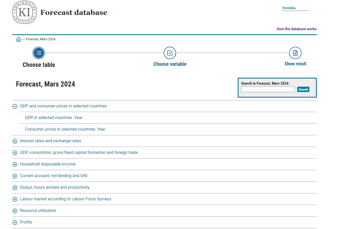
1. Select the table containing the variables of interest.
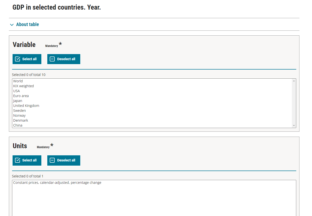
2. Using the cursor, select variables and period. Before continuing you can also customize the file format and layout of your retrieval.
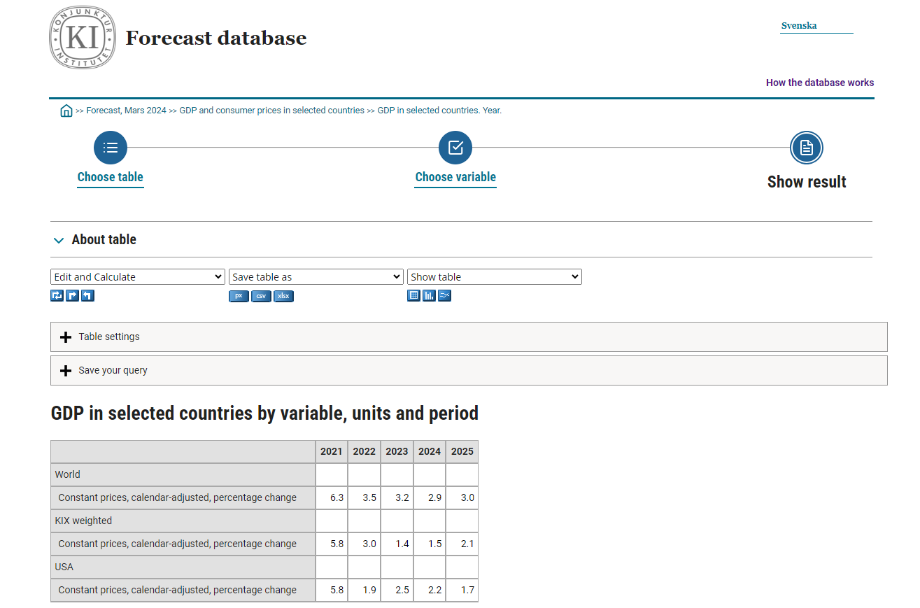
3. Your retrieval can be viewed in a number of ways, and can be exported to different file formats. It is also possible to save a link to the current query for future automatic updating. If you are programming your own retrieval solution you can get the API code for the current retrieval from the "about table" tab.
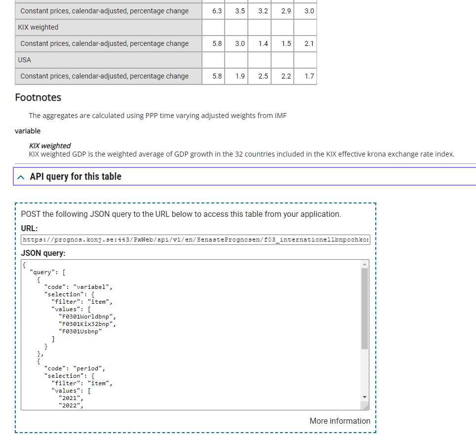
4. If you have your own application where you want to implement the extraction, you can retrieve the API code (the URL and the JSON query) by clicking on the information under "Make this table available in your application".

If a table exceeds 1,000 rows and 30 columns, not all of the table will appear on screen, but you can still download it as an Excel file or in another format. The limit for downloads is 250,000 cells

Automated data retrieval

For users who wish to integrate data collection into their own analytical workflow or software, the National Institute of Economic Research (Konjunkturinstitutet) database provides a powerful tool: an API (Application Programming Interface). The API allows you to write scripts or applications that automatically retrieve updated data from the database. You can specify exactly which information to access by defining specific variables, time periods, or data formats.

It is also possible to connect the data flow directly to your analytical environment, such as Jupyter Notebook, RStudio, or Microsoft Excel via Power Query. This enables you to schedule automated data retrievals and ensure that your models or reports always use the most recent statistics—without the need to manually access the interface each time.

The API is particularly useful when you need to repeatedly retrieve the same type of data, when performing large-scale data extractions that would otherwise require considerable manual effort, or when building automated update processes in an analysis tool, decision support system, or web service.

To get started, you should have basic programming knowledge, preferably in Python or R, which are commonly used languages in statistics and data analysis. This includes understanding how to perform API requests via HTTP, how to read and interpret responses in JSON or CSV format, and how to process tabular data structures.

Example code is available in both Python and R. You can easily copy and run the examples in your own environment. The sample scripts demonstrate how to connect to the API, retrieve a dataset, and import it into your workspace. The example also includes a simple visualization of the retrieved data, providing a quick overview of trends in the dataset. With minor modifications, you can adapt the example to design a data retrieval and analysis workflow tailored to your specific needs.

#_____________________________________________________________________________________
#
# Exempelkod för att lista tillgängliga tabeller i prognosdatabasens yta SenastePrognosen (prognos.konj.se)
# Example code for listing available tables in the "SenastePrognosen" section of the forecast database (prognos.konj.se)
#_____________________________________________________________________________________

import requests
import time

# Bas-URL till API:t där alla huvudkataloger finns
# Base URL to the API where all main directories are listed
base_url = "https://prognos.konj.se:443/PxWeb/api/v1/sv/SenastePrognosen/"

# Skicka en GET-förfrågan för att hämta huvudkatalogens innehåll
# Send a GET request to fetch the contents of the main directory
response = requests.get(base_url)
main_dirs = response.json() # Konvertera svaret till JSON / Convert response to JSON

# Loopa igenom varje objekt i huvudkatalogen
# Loop through each item in the main directory
for item in main_dirs:
if item['type'] == 'l': # Kontrollera om objektet är en katalog / Check if the item is a directory
dir_id = item['id'] # Katalogens ID / Directory ID
dir_name = item['text'] # Katalogens namn / Directory name
dir_url = base_url + dir_id + "/" # Fullständig URL till katalogen / Full URL to the directory

print(f"\n📁 Katalog: {dir_name} ({dir_id})") # Skriv ut katalogens namn / Print directory name

# Försök att hämta innehållet i katalogen upp till 3 gånger
# Try to fetch the directory contents up to 3 times
for attempt in range(3):
try:
sub_response = requests.get(dir_url) # Skicka GET-förfrågan / Send GET request
if sub_response.status_code == 200:
sub_items = sub_response.json() # Konvertera till JSON / Convert to JSON
for sub_item in sub_items:
if sub_item['type'] == 't': # Om objektet är en tabell (.px-fil) / If the item is a table
print(f" 📄 Tabell: {sub_item['text']} ({sub_item['id']})")
break # Om det lyckas, bryt loopen / If successful, break the loop
else:
print(f" ⚠️ Försök {attempt+1}: Kunde inte hämta innehåll (statuskod {sub_response.status_code})")
except Exception as e:
print(f" ⚠️ Försök {attempt+1}: Fel vid hämtning - {e}") # Fångar andra fel / Catch other errors

time.sleep(10) # Vänta 10 sekunder innan nästa försök / Wait 10 seconds before retrying

#_____________________________________________________________________________________
#
# Exempelkod för att hämta data från prognosdatabasen (prognos.konj.se)
# Example code for fetching data from the forecast database (prognos.konj.se)
#
# Du behöver installera pyjstat, skriv följande i kommandotolken
# You need to install pyjstat, in the command prompt write the following
#
# py -m pip install pyjstat
#_____________________________________________________________________________________

#_____________________________________________________________________________________

# Importera paket
# Import package
from pyjstat import pyjstat
import requests
from matplotlib import pyplot as plt
import pandas as pd

#_____________________________________________________________________________________

# Hämta årlig data från prognosdatabasen, efter att en tabell har genererats
# från databasen, är URL:en och den faktiska JSON-förfrågan belägna längst ner

# Fetch annual data from the forecast database, after a table has been generated
# from the database, the URL and the actual JSON query are located at the bottom.

# Ange URL:en
# Input the URL
POST_URL = 'https://prognos.konj.se:443/PxWeb/api/v1/sv/SenastePrognosen/f09_bnpkonsumtioninvesteringarochutrikeshandel/F0901.px'

# Ange JSON-förfrågan
# Input the JSON query
payload = {
"query": [
{
"code": "variabel",
"selection": {
"filter": "item",
"values": [
"F0901Nbnpmp"
]
}
},
{
"code": "enhet",
"selection": {
"filter": "item",
"values": [
"F"
]
}
},
{
"code": "period",
"selection": {
"filter": "item",
"values": [
"2007",
"2008",
"2009",
"2010",
"2011",
"2012",
"2013",
"2014",
"2015",
"2016",
"2017",
"2018",
"2019",
"2020",
"2021",
"2022",
"2023",
"2024",
"2025",
"2026",
"2027"
]
}
}
],
"response": {
# Observera att 'format':'px' har ändrats till JSON-stat
# Note that 'format':'px' has been changed to JSON-stat
"format": "json-stat"
}
}

#_____________________________________________________________________________________

# Ladda data
# Load data

response = requests.post(POST_URL,json = payload)
print(response)

dataset = pyjstat.Dataset.read(response.text)
df = dataset.write('dataframe')
print(df.head())

# _____________________________________________________________________________________

# Skapa graf
# Create graph

# Ändra formatet på perioden
# Change the format of the period
df["period"] = pd.to_datetime(df["period"]) #, format = "%YM%m")

# Ändra enheten från miljoner SEK till miljarder SEK för en bättre utseende i den provisoriska grafen
# Change the unit from millions SEK to billions SEK for a better appearance in the sample graph
df["value"] = df["value"] / 1000

# Skapa graf
# Create graph
plt.figure(figsize = (8,6),dpi=100)
plt.plot(df["period"],df["value"])

# Ändra bakgrundsfärg för prognosår som börjar från 2024
# Change background color for forecast years starting from 2024
plt.axvspan('2024', '2027', color='Grey', alpha=0.4, label='Highlight')
plt.figtext(0.775,0.5, 'Prognos')
plt.grid(axis = 'y', color = "lightgrey", alpha=0.3)

# Lägg till titel och visa diagramet
# Add title and show the graph

plt.title("BNP Sverige, mdkr, fasta priser \n" "2024-2027 = senaste prognosen")
plt.show()

#_____________________________________________________________________________________
#
# Exempelkod för att hämta data från statistikdabasen (statistik.konj.se)
# Example code for fetching data from the forecast database (statistik.konj.se)
#
# Du behöver installera pyjstat, skriv följande i kommandotolken
# You need to install pyjstat, in the command prompt write the following
#
# py -m pip install pyjstat
#_____________________________________________________________________________________

#_____________________________________________________________________________________

# Importera paket
# Import package
from pyjstat import pyjstat
import requests
from matplotlib import pyplot as plt
import pandas as pd

#_____________________________________________________________________________________

# Hämta månadsdata för hela perioden för variabeln Barometerindikatorn, efter att en tabell har genererats
# från databasen, är URL:en och den faktiska JSON-förfrågan belägna längst ner

# Fetch monthly data for the entire period for the variable Barometerindicator, after a table has been generated
# from the database, the URL and the actual JSON query are located at the bottom.

# Ange URL:en
# Input the URL
POST_URL = 'https://statistik.konj.se:443/PxWeb/api/v1/sv/KonjBar/indikatorer/Indikatorm.px'

# Ange JSON-förfrågan
# Input the JSON query
payload = {
"query": [
{
"code": "Indikator",
"selection": {
"filter": "item",
"values": [
"KIFI"
]
}
}
],
"response": {
# Observera att 'format':'px' har ändrats till JSON-stat
# Note that 'format':'px' has been changed to JSON-stat
"format": "json-stat"
}
}

#_____________________________________________________________________________________

# Ladda data
# Load data

response = requests.post(POST_URL,json = payload)
print(response)

dataset = pyjstat.Dataset.read(response.text)
df = dataset.write('dataframe')
print(df.head())

# _____________________________________________________________________________________

# Skapa graf
# Create graph

# Ändra formatet på perioden
# Change the format of the period

df["Period"] = pd.to_datetime(df["Period"], format = "%YM%m")
df.set_index("Period",inplace=True)

# Skapa graf
# Create graph
plt.figure(figsize = (8,6),dpi=100)
plt.plot(df[["value"]])
plt.grid(axis = 'y', color = "lightgrey", alpha=0.3)

# Lägg till titel och visa diagramet
# Add title and show the graph
plt.title("Barometerindikatorn, 1996-2024, \n" "månatlig frekvens")
plt.show()

#_____________________________________________________________________________________
#
# Exempelkod för att hämta data från statistikdabasen (statistik.konj.se) och kombinera
# ihop serier från olika uttag
# Example code for fetching data from the statistical database (statistik.konj.se) and
# combining series from different queries.
#
# Du behöver installera pyjstat, skriv följande i kommandotolken
# You need to install pyjstat, in the command prompt write the following
#
# py -m pip install pyjstat
#_____________________________________________________________________________________

#_____________________________________________________________________________________

from pyjstat import pyjstat
import requests
from matplotlib import pyplot as plt
import pandas as pd

# Hämta månadsdata för byggindustri, efter att en tabell har genererats
# från databasen, är URL:en och den faktiska JSON-förfrågan belägna längst ner

# Fetch monthly data for construction industry, after a table has been generated
# from the database, the URL and the actual JSON query are located at the bottom.

# Ange URL:en
# Input the URL
POST_URL_BYGG = 'https://statistik.konj.se:443/PxWeb/api/v1/sv/KonjBar/ftgmanad/Barboam.px'

# Ange JSON-förfrågan
# Input the JSON query
bygg_payload = {
"query": [
{
"code": "Bransch (SNI 2007)",
"selection": {
"filter": "item",
"values": [
"BBYG"
]
}
},
{
"code": "Fråga",
"selection": {
"filter": "item",
"values": [
"106"
]
}
},
{
"code": "Serie",
"selection": {
"filter": "item",
"values": [
"S"
]
}
}
],
"response": {
# Observera att 'format':'px' har ändrats till JSON-stat
# Note that 'format':'px' has been changed to JSON-stat
"format": "json-stat"
}
}

# Ladda data, mm
# Load data, etc
response_bygg = requests.post(POST_URL_BYGG,json = bygg_payload)
print(response_bygg)
dataset_bygg = pyjstat.Dataset.read(response_bygg.text)
df_bygg = dataset_bygg.write('dataframe')
df_bygg["Period"] = pd.to_datetime(df_bygg["Period"], format = "%YM%m")

#_____________________________________________________________________________________

# Återupprepa datauttaget för ytterligare tre serier
# Repeat the data extraction for three additional series

# Handeln
# Trade

POST_URL_HANDEL = 'https://statistik.konj.se:443/PxWeb/api/v1/sv/KonjBar/ftgmanad/Barhanm.px'

handel_payload = {
"query": [
{
"code": "Bransch (SNI 2007)",
"selection": {
"filter": "item",
"values": [
"BHAN"
]
}
},
{
"code": "Fråga",
"selection": {
"filter": "item",
"values": [
"104"
]
}
},
{
"code": "Serie",
"selection": {
"filter": "item",
"values": [
"S"
]
}
}
],
"response": {
"format": "json-stat"
}
}

response_handel = requests.post(POST_URL_HANDEL,json = handel_payload)
print(response_handel)
dataset_handel = pyjstat.Dataset.read(response_handel.text)
df_handel = dataset_handel.write('dataframe')
df_handel["Period"] = pd.to_datetime(df_handel["Period"], format = "%YM%m")

# Tillverkningsindustri
# Manufacturing industry

POST_URL_TILLV = 'https://statistik.konj.se:443/PxWeb/api/v1/sv/KonjBar/ftgmanad/Barindm.px'

payload_tillv = {
"query": [
{
"code": "Bransch (SNI 2007)",
"selection": {
"filter": "item",
"values": [
"BTVI"
]
}
},
{
"code": "Fråga",
"selection": {
"filter": "item",
"values": [
"107"
]
}
},
{
"code": "Serie",
"selection": {
"filter": "item",
"values": [
"S"
]
}
}
],
"response": {
"format": "json-stat" # <- Notera att jag ändrat från px till json-stat för att kunna läsa in
}
}

response_tillv = requests.post(POST_URL_TILLV,json = payload_tillv)
print(response_tillv)
dataset_tillv = pyjstat.Dataset.read(response_tillv.text)
df_tillv = dataset_tillv.write('dataframe')
print(df_tillv.head())
df_tillv["Period"] = pd.to_datetime(df_tillv["Period"], format = "%YM%m")

# Tjänstesektorn
# Service sector

POST_URL_TJANST = 'https://statistik.konj.se:443/PxWeb/api/v1/sv/KonjBar/ftgmanad/Bartjam.px'

payload_tjanst = {
"query": [
{
"code": "Bransch (SNI 2007)",
"selection": {
"filter": "item",
"values": [
"BTJA"
]
}
},
{
"code": "Fråga",
"selection": {
"filter": "item",
"values": [
"105"
]
}
},
{
"code": "Serie",
"selection": {
"filter": "item",
"values": [
"S"
]
}
}
],
"response": {
"format": "json-stat" # <- Notera att jag ändrat från px till json-stat för att kunna läsa in
}
}

response_tjanst = requests.post(POST_URL_TJANST,json = payload_tjanst)
print(response_tillv)
dataset_tjanst = pyjstat.Dataset.read(response_tjanst.text)
df_tjanst = dataset_tjanst.write('dataframe')
print(df_tjanst.head())
df_tjanst["Period"] = pd.to_datetime(df_tjanst["Period"], format = "%YM%m")

# _____________________________________________________________________________________

# Skapa graf
# Create graph

plt.figure(figsize = (8,6),dpi=100)

plt.plot(df_bygg["Period"],df_bygg["value"],label = df_bygg["Bransch (SNI 2007)"].loc[0])
plt.plot(df_handel["Period"],df_handel["value"],label = df_handel["Bransch (SNI 2007)"].loc[0])
plt.plot(df_tillv["Period"],df_tillv["value"],label = df_tillv["Bransch (SNI 2007)"].loc[0])
plt.plot(df_tjanst["Period"],df_tjanst["value"],label = df_tjanst["Bransch (SNI 2007)"].loc[0])

plt.axhline(0, linestyle = "--", color="grey", lw =1)
plt.grid(axis = 'y', color = "lightgrey", alpha=0.3)

plt.legend()

plt.title("Antal anställda (utfall), nettotal, 1996-2024, \n" "månatlig frekvens")
plt.show()

#_____________________________________________________________________________________
#
# Exempelkod för att hämta data från prognosdatabasen (prognos.konj.se)
# Example code for fetching data from the forecast database (prognos.konj.se)
#
# Du behöver installera olika paket
# You need to install additional packages
#
# install.packages("httr")
# install.packages("rjstat")
# install.packages("ggplot2", repos="https://cran.r-project.org/")
#_____________________________________________________________________________________

# Importera paket
# Import package
library(httr)
library(ggplot2)
library(rjstat)

# Ange URL:en
# Input the URL
POST_URL <- 'https://prognos.konj.se:443/PxWeb/api/v1/sv/SenastePrognosen/f09_bnpkonsumtioninvesteringarochutrikeshandel/F0901.px'

# Ange JSON-förfrågan
# Input the JSON query
payload <- '{
"query": [
{
"code": "variabel",
"selection": {
"filter": "item",
"values": [
"F0901Nbnpmp"
]
}
},
{
"code": "enhet",
"selection": {
"filter": "item",
"values": [
"F"
]
}
},
{
"code": "period",
"selection": {
"filter": "item",
"values": [
"2007",
"2008",
"2009",
"2010",
"2011",
"2012",
"2013",
"2014",
"2015",
"2016",
"2017",
"2018",
"2019",
"2020",
"2021",
"2022",
"2023",
"2024",
"2025",
"2026",
"2027"
]
}
}
],
"response": {
"format": "json-stat"
}
}'

#_____________________________________________________________________________________

# Ladda data
# Load data

req <-POST(POST_URL, body=payload,encode = "json")
str(req$status) # Get status code, 200 = ok
df <- fromJSONstat(content(req, "text"))

# _____________________________________________________________________________________

# Skapa graf
# Create graph

final_df <- df[[1]]
final_df$value <- final_df$value / 1000

plot <- ggplot(final_df,aes(x=period,y=value,group=1))+
geom_rect(
aes(xmin = 18, xmax = 21, ymin = -Inf, ymax = Inf),
fill = "lightgrey",
alpha = 0.2)+
geom_line(color="blue",linewidth=1,alpha=0.8,linetype=1)+
labs(
title= "BNP Sverige, mdkr, fasta priser, \n2024-2027 = senaste prognosen",
x = "",
y = ""
)+
theme(
# Hide panel borders and remove grid lines
panel.background = element_rect(fill = 'white'),
panel.grid.major.y = element_line(colour="lightgrey"),
# Change axis line
axis.line = element_line(colour = "black"))+
annotate("text", 19.5, y=5250, label= "prognos")

print(plot)

#_____________________________________________________________________________________
#
# Exempelkod för att hämta data från statistikdabasen (statistik.konj.se)
# Example code for fetching data from the forecast database (statistik.konj.se)
#
# Du behöver installera olika paket
# You need to install additional packages
#
# install.packages("httr")
# install.packages("rjstat")
# install.packages("ggplot2", repos="https://cran.r-project.org/")
#_____________________________________________________________________________________

# Importera paket
# Import package
library(httr)
library(ggplot2)
library(rjstat)

# Ange URL:en
# Input the URL
POST_URL <- 'https://statistik.konj.se:443/PxWeb/api/v1/sv/KonjBar/indikatorer/Indikatorm.px'

# Ange JSON-förfrågan
# Input the JSON query
payload <- '{
"query": [
{
"code": "Indikator",
"selection": {
"filter": "item",
"values": [
"KIFI"
]
}
}
],
"response": {
"format": "json-stat"
}
}'

#_____________________________________________________________________________________

# Ladda data
# Load data

req <-POST(POST_URL, body=payload,encode = "json")
str(req$status) # Get status code, 200 = ok
df <- fromJSONstat(content(req, "text"))

req <-POST(POST_URL, body=payload,encode = "json")
str(req$status) # Get status code, 200 = ok
df <- fromJSONstat(content(req, "text"))
final_data <- df[[1]]

# _____________________________________________________________________________________

# Skapa graf
# Create graph

final_data$Period<-gsub("M","-",as.character(final_data$Period))
final_data$Period<-gsub(" ","",paste(final_data$Period,"-01"))
final_data$Period<-as.Date(final_data$Period,format="%Y-%m-%d")

plot <- ggplot(final_data,aes(y=value,x=Period))+
geom_line(color="blue",linewidth=1,alpha=0.8,linetype=1)+
scale_x_date(
limits = as.Date(c('1996-01-01','2024-01-01')),
breaks = scales::date_breaks("2 years"), date_labels="%Y",
guide = guide_axis(angle = 45)
)+
scale_y_continuous(limits=c(60,130),
breaks = scales::breaks_width(10)
)+
theme(
# Hide panel borders and remove grid lines
panel.background = element_rect(fill = 'white'),
panel.grid.major.y = element_line(colour="lightgrey"),
# Change axis line
axis.line = element_line(colour = "black")
)+
labs(
title="Barometerindikatorn, 1996-2024, \månatlig frekvens"

)
print(plot)

#_____________________________________________________________________________________
#
# Exempelkod för att hämta data från statistikdabasen (statistik.konj.se) och kombinera
# ihop serier från olika uttag
# Example code for fetching data from the statistical database (statistik.konj.se) and
# combining series from different queries.
#
# Du behöver installera olika paket
# You need to install additional packages
#
# install.packages("httr")
# install.packages("rjstat")
# install.packages("ggplot2", repos="https://cran.r-project.org/")
#_____________________________________________________________________________________

# Importera paket
# Import package
library(httr)
library(ggplot2)
library(rjstat)

# Ange URL:en
# Input the URL

# BYGG
POST_URL_BYGG = 'https://statistik.konj.se:443/PxWeb/api/v1/sv/KonjBar/ftgmanad/Barboam.px'

# Ange JSON-förfrågan
# Input the JSON query
bygg_payload = '{
"query": [
{
"code": "Bransch (SNI 2007)",
"selection": {
"filter": "item",
"values": [
"BBYG"
]
}
},
{
"code": "Fråga",
"selection": {
"filter": "item",
"values": [
"106"
]
}
},
{
"code": "Serie",
"selection": {
"filter": "item",
"values": [
"S"
]
}
}
],
"response": {
"format": "json-stat"
}
}'

# Ladda data, mm
# Load data, etc
req_bygg <-POST(POST_URL_BYGG, body=bygg_payload,encode = "json")
str(req_bygg$status) # Get status code, 200 = ok
df_bygg <- fromJSONstat(content(req_bygg, "text"))
final_data_bygg <- df_bygg[[1]]
final_data_bygg$Period<-gsub("M","-",as.character(final_data_bygg$Period))
final_data_bygg$Period<-gsub(" ","",paste(final_data_bygg$Period,"-01"))
final_data_bygg$Period<-as.Date(final_data_bygg$Period,format="%Y-%m-%d")

#_____________________________________________________________________________________

# Återupprepa datauttaget för ytterligare tre serier
# Repeat the data extraction for three additional series

# Handeln
# Trade

POST_URL_HANDEL = 'https://statistik.konj.se:443/PxWeb/api/v1/sv/KonjBar/ftgmanad/Barhanm.px'

handel_payload = '{
"query": [
{
"code": "Bransch (SNI 2007)",
"selection": {
"filter": "item",
"values": [
"BHAN"
]
}
},
{
"code": "Fråga",
"selection": {
"filter": "item",
"values": [
"104"
]
}
},
{
"code": "Serie",
"selection": {
"filter": "item",
"values": [
"S"
]
}
},
{
"code": "Period",
"selection": {
"filter": "all",
"values": [
"*"
]
}
}
],
"response": {
"format": "json-stat"
}
}'

req_handel <-POST(POST_URL_HANDEL, body=handel_payload,encode = "json")
str(req_handel$status) # Get status code, 200 = ok
df_handel <- fromJSONstat(content(req_handel, "text"))
final_data_handel <- df_handel[[1]]
final_data_handel$Period<-gsub("M","-",as.character(final_data_handel$Period))
final_data_handel$Period<-gsub(" ","",paste(final_data_handel$Period,"-01"))
final_data_handel$Period<-as.Date(final_data_handel$Period,format="%Y-%m-%d")

# Tillverkningsindustri
# Manufacturing industry

POST_URL_TILLV = 'https://statistik.konj.se:443/PxWeb/api/v1/sv/KonjBar/ftgmanad/Barindm.px'

payload_tillv = '{
"query": [
{
"code": "Bransch (SNI 2007)",
"selection": {
"filter": "item",
"values": [
"BTVI"
]
}
},
{
"code": "Fråga",
"selection": {
"filter": "item",
"values": [
"107"
]
}
},
{
"code": "Serie",
"selection": {
"filter": "item",
"values": [
"S"
]
}
},
{
"code": "Period",
"selection": {
"filter": "all",
"values": [
"*"
]
}
}
],
"response": {
"format": "json-stat"
}
}'

req_tillv <-POST(POST_URL_TILLV, body=payload_tillv,encode = "json")
str(req_tillv$status) # Get status code, 200 = ok
df_tillv <- fromJSONstat(content(req_tillv, "text"))
final_data_tillv <- df_tillv[[1]]
final_data_tillv$Period<-gsub("M","-",as.character(final_data_tillv$Period))
final_data_tillv$Period<-gsub(" ","",paste(final_data_tillv$Period,"-01"))
final_data_tillv$Period<-as.Date(final_data_tillv$Period,format="%Y-%m-%d")

# Tjänstesektorn
# Service sector

POST_URL_TJANST = 'https://statistik.konj.se:443/PxWeb/api/v1/sv/KonjBar/ftgmanad/Bartjam.px'

payload_tjanst = '{
"query": [
{
"code": "Bransch (SNI 2007)",
"selection": {
"filter": "item",
"values": [
"BTJA"
]
}
},
{
"code": "Fråga",
"selection": {
"filter": "item",
"values": [
"105"
]
}
},
{
"code": "Serie",
"selection": {
"filter": "item",
"values": [
"S"
]
}
},
{
"code": "Period",
"selection": {
"filter": "all",
"values": [
"*"
]
}
}
],
"response": {
"format": "json-stat"
}
}'

req_tjanst <-POST(POST_URL_TJANST, body=payload_tjanst,encode = "json")
str(req_tjanst$status) # Get status code, 200 = ok
df_tjanst <- fromJSONstat(content(req_tjanst, "text"))
final_data_tjanst <- df_tjanst[[1]]
final_data_tjanst$Period<-gsub("M","-",as.character(final_data_tjanst$Period))
final_data_tjanst$Period<-gsub(" ","",paste(final_data_tjanst$Period,"-01"))
final_data_tjanst$Period<-as.Date(final_data_tjanst$Period,format="%Y-%m-%d")

# _____________________________________________________________________________________

# Skapa graf
# Create graph

test_merge <- merge(final_data_bygg,final_data_handel, on = "Bransch (SNI 2007)", all = T)
test_merge <- merge(test_merge, final_data_tillv, on = "Bransch (SNI 2007)", all = T)
test_merge <- merge(test_merge, final_data_tjanst, on = "Bransch (SNI 2007)", all = T)
names(test_merge)[names(test_merge) == "Bransch (SNI 2007)"] <- "Bransch"

plot <- ggplot(test_merge, aes(x=Period,y=value,group = Bransch,color=Bransch)) + geom_line(lwd=1) +
theme(
# Hide panel borders and remove grid lines
panel.background = element_rect(fill = 'white'),
panel.grid.major.y = element_line(colour="lightgrey"),
# Change axis line
axis.line = element_line(colour = "black"),
legend.position = c(0.87,0.1),
legend.background=element_rect(colour="lightgrey"),
)+
scale_x_date(
limits = as.Date(c('2000-01-01','2024-01-01')),
breaks = scales::date_breaks("2 years"), date_labels="%Y",
guide = guide_axis(angle = 45)
)+
labs(
title="Barometerindikatorn, 1996-2024, \nmånatlig frekvens",
y = "",
x = ""
)
print(plot

How the databases work

Automated data retrieval

Example code 1 in Python for the forecast database – fetch data

Example code 2 in Python for the forecast database – fetch data

Example code 3 in Python for the statistics database – fetch data

Example code 4 in Python for the statistics database – fetch data

Example code 5 in R for the forecast database – fetch data

Example code 6 in R for the statistics database – fetch data

Example code 7 in R for the statistics database – fetch data